Optimum Exposure Times

This tends to be a “Holy Grail” kind of topic. I have experienced far too many evenings where I have imaged for hours, but the sky glow corrupted the images so badly that they were not usable. I end up asking myself, “Would a longer exposure have been a better choice?” or “Was this just a night to keep the telescope in the house?

I decided that I need to research this subject more. I have read lots about “swamping the Read Noise,” which sounds like a good scheme. If I use my OPTOLONG L-eNhance filter at my dark site, I found that the “swamp the Read Noise” approach indicated that, because of the very low sky background, I needed ridiculously long exposure times …so I keep looking. Longer exposures typically have better SNR, but longer exposures have several issues…

a)The Sky Glow can become excessive.
b)Too many stars become saturated.
Issues like differential flexure, poor polar alignment, and poor guiding cause stars to become oblong, and fine details are smeared. These specific issues are well documented, and I’m going to assume that you have either already eliminated these issues or that you are looking for something else to improve your astrophotography.

Let’s start by documenting some camera issues that are well understood…Bias and Dark Current

BIAS
Every camera has Bias. As with most camera issues, Bias can be described as having two components: signal and random noise. The signal component of BIAS can be isolated for a camera by generating a masterBIAS frame. Several BIAS frames are taken and then averaged together to obtain a master BIAS frame. Only the persistent signal survives this averaging. The random noise is strongly attenuated and, for a masterBIAS, can be considered eliminated.

When you display your masterBIAS with CaLIGHTs, your first reaction will be “why is it still noisy?” The BIAS signal is a collection of small offsets that are unique and persistent for each pixel. When you look at a masterBIAS, all of these unique offsets will appear as noise. For my QHY294C astroCAM, its GAIN=1600 masterBIAS has FITS file values with a mean value of 22 counts and a standard deviation of 1.73 counts.

The random noise component of BIAS has been given a name which is Read Noise. Most camera manufacturers provide graphs indicating the Read Noise as a function of the camera system gain. For my QHY294C, the Read Noise is 1.63e- at a GAIN setting of 1600. A camera GAIN of 1600 is equivalent to a camera system gain of 0.872 e-/ADU(14b). I want to relate this value to the values that are stored in my FITS files. The QHY software multiplies the 14bit values by 4 so that they are effectively 16bit values. This causes the camera system gain to be divided by 4 yielding a value of 0.218e/count(16b). This allows me to convert the Read Noise value of 1.63e- to an equivalent FITS file value of 1.63/0.218 = 7.5 counts.

DARK Current
Another dominant camera issue is called DARK Current, which also has a signal and a random noise component. We can isolate the DARK Current signal component by generating a masterDARK using the same averaging technique, only this time, with DARK frames. The masterDARK contains the BIAS signal and the DARK Current signal. The DARK Current signal is more complicated than the BIAS signal. While DARK Current is also a collection of small offsets which are unique and persistent for each pixel…these offsets increase with both exposure time and camera temperature. There is also a phenomenon called Amp Glow, which is a sub-component of DARK Current.

The method developed for dealing with DARK Current is to build a library of masterDARKs. DARK frames are taken at several exposure lengths and camera temperatures. DARK frames taken at the same exposure length and camera temperatures are then combined to build a masterDARK library. My DARK library includes a series of masterDARKs for camera temperature of -10 Celsius and 0 Celsius, and GAIN settings of 1600 and 2500. This DARK Library contains masterDARKs for exposure times of 200, 300, 450, and 600 seconds. For my QHY294C astroCAM, at a GAIN of 1600, camera temperature of 0 Celsius, and exposure of 600 seconds, the masterDARK has FITS file values with a mean value of 100 counts and a standard deviation of 17 counts. I put together a graph that compares the mean and standard deviation values for the GAIN = 1600 masterDARKs in my DARK library.

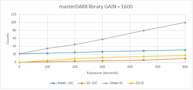
While these masterDARKs do a great job of eliminating the Dark Current signal in my astrophotos, I also know that there is a Dark Current random noise component that can be just as significant as the Read noise. This DARK Current noise also varies with exposure length and camera temperature.

When I calibrate my LIGHT frames using a masterDARK, I know that this eliminates the BIAS signal and the DARK Current signal. Unfortunately, it does not eliminate the Read noise or the DARK Current noise. I think that DARK Current noise is very significant, but it’s the Read Noise that seems to get all the attention. I decided to generate a graph to help explain what I mean. I only used the DARK frames and masterDARKs for a camera GAIN of 1600. For each exposure and camera temperature, I used a corresponding DARK frame and masterDARK. CaLIGHTs subtracted the masterDARK from the DARK frame, which leaves only the camera random noise. The camera random noise is composed of Read Noise and DARK Current noise. I used CaLIGHTs to generate standard deviation values, which are shown here.

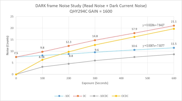
The two dotted lines are the Camera noise in my DARK frames. The red dotted line is for zero Celsius…the blue dotted line is for -10 Celsius. I included the Read Noise datapoint (7.5 counts) because a BIAS frame is essentially a zero-second DARK frame. I was surprised to see that these dotted lines are straight. I included the equations that best fit these two dotted lines.
Adding or subtracting standard deviations is done by squaring the values. So a valid equation for calculating the camera noise is as follows:

CameraNoise^2 = ReadNoise^2 + DarkCurrentNoise^2

Re-arranging terms gives us…

DarkCurrentNoise = \sqrt{\smash[b]{CameraNoise^2 - ReadNoise^2}}

For the 300 second exposures I get the following

DarkCurrentNoise(0C) =  \sqrt{\smash[b]{14.8^2 - 7.5^2}} = 12.75\ \ counts

DarkCurrentNoise(-10C) =  \sqrt{\smash[b]{9.6^2 - 7.5^2}} = 6.0\ \ counts

For the 600 second exposures I get the following

DarkCurrentNoise(0C) =  \sqrt{\smash[b]{21.1^2 - 7.5^2}} = 19.7\ \ counts

DarkCurrentNoise(-10C) =  \sqrt{\smash[b]{11.5^2 - 7.5^2}} = 8.7\ \ counts

I went ahead and calculated the Dark Current noise for all of the data points and added them to my graph. The solid orange line in the graph is what the DARK Current noise is at zero Celsius. The solid grey line is what the DARK Current noise is at -10 Celsius. I was happy to see that these solid lines are not straight. This tells me that DARK Current noise looks like a type of Poisson or Shot noise. Poisson or Shot noise increases with the square root of the signal magnitude. Camera manufacturers always show graphs that indicate that DARK Current increases at a constant rate for any given camera temperature. To me, this means that DARK Current noise increases with the square root of the exposure time. The solid orange and grey lines do look a bit like a square root…but not exactly.

Hopefully, from my graph, you can clearly see that the noise contributed by Dark Current can be significantly larger than your camera’s Read noise. You can convert these noise values to electrons by multiplying them by 0.218.

“Swamp the Read Noise” Method
The “swamp the read noise” calculation asks us to determine an exposure time where the noise introduced by sky glow “swamps” the read noise of the camera. This is a practical approach that only requires knowing the camera’s read noise. I think you can now understand that a more specific question is “At what exposure time will the noise introduced by sky glow ‘swamp’ the camera noise.

So let’s look at what is meant by “swamp”. There is a cloudy nights topic that describes a “swamp factor”. Here is the link
https://www.cloudynights.com/topic/632988-exposure-times/?p=8827783
An equation is presented that calculates how the “swamp factor” relates to how the sky glow noise dominates the total noise in a LIGHT frame. Here is what this equation tells us.

You can see how increasing the swamp factor causes the Sky Glow Noise to dominate the noise in a LIGHT frame. You can also see that when the swamp factor gets beyond a value of 3 that the sky glow noise dominance is pretty much established. A swamp factor of 3 is quoted as being a minimum exposure criterion to aim for, so let’s see how that works.

At a GAIN of 1600, my QHY294C has a read noise of 1.63e- which is equivalent to 7.5 counts. In order to achieve a swamp factor of 3, I need to achieve LIGHT frames where the noise in a dark area that is devoid of stars and deep sky objects(DSOs) needs to be 3 x 7.5 = 22.5 counts or greater. I can easily determine the noise in my LIGHT frames using CaLIGHTs.

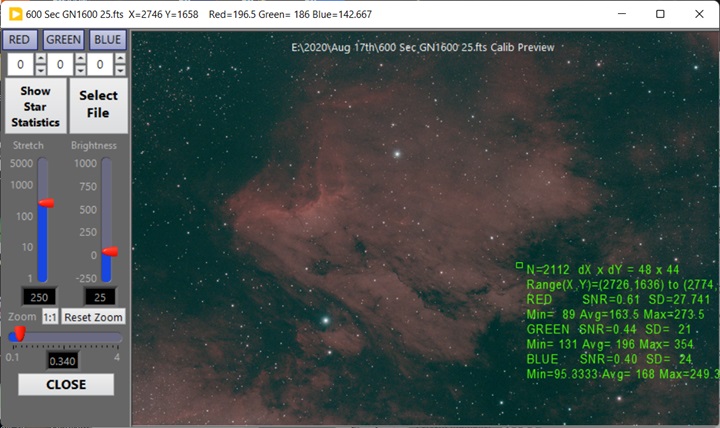
As an example, I called up a LIGHT frame I took in August of 2020 of the Pelican Nebula using CaLIGHTs. I was using a camera GAIN of 1600 and a camera temperature of zero Celsius. I also used a masterDARK, which eliminates the BIAS and DARK Current signals but does not remove the Read noise or the DARK Current noise. Here I have right-clicked and dragged a small box of dark pixels as close to the centre of the image as I can find. Because this rectangle is devoid of stars and nebulosity, I consider it to be a good example for evaluating the sky background. The green text contains lots of statistics about the red, green, and blue pixels within this small green box. The SD values are the standard deviations for the red, green, and blue pixels. So the 27.741, 21, and 24 values are very close to 22.5, so I barely achieved the swamp factor of 3. You may also have noticed that this is a 600-second exposure, so calling it a minimum exposure length is an eye-opener. This is just “par for the course” when using a narrowband filter. Here I was using an OPTOLONG L-eNhance narrowband filter.

So I was able to swamp the read noise, but I know that the camera noise can be much more than read noise. According to my DARK frame Noise Study, a 600-second DARK frame with a camera temperature of zero Celsius will have a camera noise of 21.1 counts. In order to achieve a total camera noise swamp factor of three, I would need the total noise in my LIGHT frames to be larger than 3 x 21.1 = 63.3 counts…Yiks!!! To compare what this means, I prepared this graph that shows the swamp factor using read noise and how it changes if I use total camera noise.

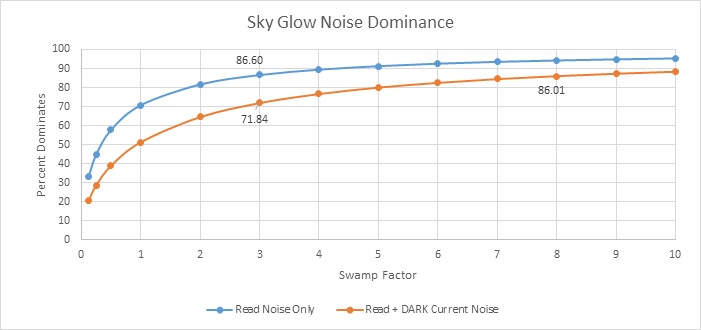
The way to interpret this graph is that the blue curve is the Sky Glow Noise Dominance when considering only the read noise. The orange curve is the percent dominance when considering the Total Camera Noise in a 600-second exposure at zero Celsius and GAIN = 1600. The swamp factor shown along the X axis only applies to the “Read Noise Only” curve.

So when I am using a swamp factor of 3x Read Noise, I might believe the Sky Glow Noise dominates the camera noise by 86.60 percent. When considering that camera noise also includes DARK Current noise, the Sky Glow Noise only dominates the camera noise by 71.84 percent. I would need to achieve a swamp factor of 8 x Read Noise before the Sky Glow Noise would dominate the camera noise by 86.01 percent. When the camera is cooled to a lower temperature, the difference between the two curves becomes less. This is good news for cooled astroCAM users… It’s bad news for uncooled DSLR users imaging on a warm summer’s evening. So it’s a minimum goal to swamp the read noise by a factor of 3. Hopefully, you can see why swamping the read noise by 10 times is highly suggested.

When I first read about the “swamp the read noise” method, it almost convinced me that sky glow noise is a good thing. I want to take photos that have as little noise as possible! Imaging from my dark site is great because Sky Glow is minimized. I have always thought there is a relationship between Sky Glow noise and the optimum exposure length. I read a great write-up on the Sharpcap forum posted by Dr. Robin Glover. https://forums.sharpcap.co.uk/viewtopic.php?t=456

I am going to build on his write-up by including my findings regarding DARK Current noise. I am also going to avoid talking about electrons and photons and try to focus solely on the count values in my fits files. This analysis is going to assume that you are using masterDARKs when you calibrate your LIGHT frames. The masterDARK will remove the effects of BIAS and DARK Current, but will not remove the DARK Current noise or the Read noise because both these noise sources are random in nature.

So let’s define some parameters:
Note: All noise values are standard deviation values. Their units are counts.
T = Total integration time of all the subframes. This easily adds up to hours. Units are seconds
R = Read noise. Units are counts.
K= Dark Current noise rate. Units are counts/second K=0.0228 @ 0C and K= 0.0067 @ -10C for my QHY294C
t = Subframe exposure time. All the subframes have the same exposure length. Units are seconds

C= Camera Noise. Units are counts. The equation for C is as follows:

C  = K*t + R 

This equation for camera noise is true for my QHY294C. You will need to figure out this equation for your camera. Let’s keep going and derive some equations for Sky Glow…

S = Sky Glow noise. Units are counts. Tricky to calculate!
s = Sky Glow rate. This is the rate at which Sky Glow builds up in our astrophotos. Units are counts/second.
E = This is the camera system gain(16b). For my QHY294C at GAIN = 1600, E = 0.218 electrons/count. Units are e-/count

Sky Glow is considered to be a Poisson noise source. Calculating the noise introduced by Poisson(shot) noise sources forces us to temporarily convert count values to electrons and finally back to counts. This is because translating the Sky Glow magnitude to its corresponding Poisson noise requires the values to be in electrons. So let’s create an equation for Sky Glow noise.

Poisson noise = sqrt(N); where N is the magnitude. All values must be in electrons…it took weeks for me to realize this. Many thanks to Dr. Robin Glover for explaining this to me.

SkyGlowMagnitude(counts) = s*t

SkyGlowNoise(counts)=S=\frac{\sqrt{\smash[b]{s*t*E}}} E

Let’s put together an equation that tells us what the total noise will be for the sky glow in a single LIGHT frame taken at 0 Celsius:

TotalNoise(n)=\sqrt{\smash[b]{C^2+S^2}}

Substituting equations for C and S

TotalNoise(n)=\sqrt{\smash[b]{(K*t+R)^2+\frac{s*t} {E}}}

Once we have taken our LIGHT frames, the next step is to stack them. Let’s put together an equation that tells us what the Total Noise is after stacking.

TotalNoise=\sqrt{\smash[b]{\frac{T} {t}}} * TotalNoise(n)

where T / t = # of LIGHT frames. Substituting for TotalNoise(n) gives us…

TotalNoise=\sqrt{\smash[b]{\frac{T} {t}}} * \sqrt{\smash[b]{(K*t+R)^2+\frac{s*t} {E}}}

Boy…this is looking ugly.

SNR – Signal to Noise Ratio

At this point, I am going to introduce the concept of signal-to-noise ratio [SNR]. For our stacked image…

SNR=\frac {TotalSignal} {TotalNoise}

SNR is useful for determining the quality of any part of an image. The higher the SNR, the clearer the details and the smoother the dark background.

Let’s figure out what the SNR equation is for any small section of a DSO. Just like Sky Glow, light generated by a DSO is a Poisson(Shot) noise source, which contributes to the total noise in the image. A DSO has a rate at which counts build up in our astrophotos. Let’s define the following terms for the DSO:

d = DSO rate. Units are counts/second. This rate depends on what part of the DSO you are interested in. Here I am concerned with the faintest sections which are always the toughest to extract any detail.
DSOTotalSignal = d x T ;Units are counts
D = DSO noise. ;Units are counts

D=\frac{\sqrt{\smash[b]{d*t*E}}} E

SNR=\frac{d*T} {\sqrt{\smash[b]{\frac{T} {t}}} * \sqrt{\smash[b]{(K*t+R)^2+\frac{s*t} {E}+\frac{d*t} {E}}}}

I am going to try and simplify this equation. If I substitute…

T=\sqrt{\smash[b]{T}} *\sqrt{\smash[b]{T}}

and

\sqrt{\smash[b]{\frac{T} {t}}}=\frac{\sqrt{\smash[b]{T}}} {\sqrt{\smash[b]{t}}}

this causes the equation to become…

SNR=\frac{\sqrt{\smash[b]{T}}*d*\sqrt{\smash[b]{t}}} {\sqrt{\smash[b]{(K*t+R)^2+\frac{(s+d)*t} {E}}}}

I want to graph something, but I need to figure out a good value for “s”. I am going to revisit the SD values I extracted from the 600-second Pelican Nebula LIGHT frame I presented earlier in this post. The camera temperature was zero degrees Celsius, and the DARK Frame Noise Study graph indicates that the camera noise would be 21.1 counts. The SD values for the red, green, and blue pixels were 27.741, 21, and 24, respectively. I am going to use a value of 24 to represent the total noise in this LIGHT frame. I can now calculate the Sky Glow noise.

SkyGlowNoise=\sqrt{\smash[b]{24^2 - 21.1^2}} = 11.4 \thinspace counts

I can calculate a Sky Glow Magnitude as follows:

SkyGlowMagnitude=\frac{(11.4*0.218)^2} {0.218}=28.33\space counts

I can now determine the Sky Glow Rate=SkyGlowMagnitude/ExposureTime

SkyGlowRate = s =\frac{28.33} {600}=0.047\space \frac{counts}{second}

I am going to use a value of 0.05 counts per second for the graph. For simplicity, I am also going to use a DSO rate of 0.05 counts per second.

This graph shows how exposure length influences the SNR of the DSO. This is for the case where you only have time for one hour of exposure. The camera GAIN=1600 and camera temperature=0 Celsius. The Read noise is 7.5 counts(1.63e-), Sky Glow rate and DSO rate are both 0.05 counts per second. Each LIGHT frame would have been calibrated using a masterDARK so that BIAS and DARK Current were eliminated…leaving only Read noise and DARK Current noise. The blue “Noise(n)” trace shows what the total noise is for each exposure time. The total noise is the summation of all the random noise components of DSO, Sky Glow, BIAS, and DARK Current. The orange “SNR(n)” trace is what the SNR is for each exposure time. The grey “SNR” trace is what the SNR will be for the DSO in the stacked image.

The orange “SNR(n)” trace is interesting because it tells me that the SNR of a single LIGHT frame will always be improved if I use longer exposure times. I had always thought that longer exposures were the “best practice” for astrophotography.

The grey “SNR” trace is extremely interesting because it tells me that there is an optimum exposure time. Very short exposures have low SNR values because of the “swamp the Read noise” issue. You can also clearly see that the SNR value reaches its maximum at 330 seconds and starts decreasing for exposures higher than 330 seconds. This slow SNR decrease happens because of DARK Current noise. DARK Current noise is very significant for uncooled cameras such as DSLRs.

Which is better…5 x 200 seconds or 2 x 500 seconds?
Much has been written about statements like “which is better…5 x 200 seconds or 2 x 500 seconds?” My DSO SNR graph indicates that there is an optimum exposure length, and it is governed by Read noise for short exposures and DARK Current noise for long exposures. Increased cooling makes this long exposure issue all but go away, so uncooled DSLR users should pay attention to this phenomenon.

I calculated the DARK Current noise for an ASI2600MC Pro camera in this post https://astrohobby.ca/2022/01/17/extracting-camera-performance-data-using-calights-v3-1-6/. This camera is advertised as having very low DARK Current…but…it does have similar DARK Current noise to my QHY294C. I commented on this finding towards the end of that post. I think that as long as any astroCAM is cooled to -10 or lower, the DARK Current noise will be low enough that longer exposures will always yield higher SNR in your stacked images. Maybe someday I will be able to study the ASI2600MC Pro more closely.

Teasing out the important trends

Because I used an Excel spreadsheet, I was able to vary some of the parameters to see what happens.

-I varied the available time from 30 minutes up to 4 hours, with the 330-second exposure always yielded the highest SNR in the stacked result. A longer available time always yielded a higher SNR.

-I also varied the Sky Glow from 0.05 up to 4 counts/second, and the 330-second exposure time, once again, had the highest SNR in the stacked result. Increasing Sky Glow significantly decreased the overall SNR, which is the phenomenon I am all too familiar with.

-When I halved the Read noise to 3.75 counts(0.815e-), the SNR quickly rose to 3.35 with the optimum exposure time decreasing to 180 seconds, but the SNR slowly decreased for higher exposures. When I doubled the Read noise to 15 counts(3.26e-), the SNR slowly rose upwards to only 2.22 with the optimum exposure time occurring at 660 seconds.

-I changed the camera DARK Current noise by changing the camera temperature from zero Celsius to -10 Celsius. At zero Celsius, the optimum 330-second exposure yielded a maximum stacked SNR of 2.81. At -10 Celsius, the SNR quickly rose above 3.0, with a 330-second exposure yielding a stacked SNR of 3.48, and didn’t reach its optimum SNR of 3.69 until an exposure time of 1100 seconds. When I modified the DARK Current noise equation to simulate double the DARK Current noise, the maximum stacked SNR only reached 2.22 with the optimum exposure time decreasing to 180 seconds. After reaching the maximum stacked SNR, it dropped off far quickly as the exposure time increased. In summary:

-Total available imaging time does not change the optimum exposure time.
–The amount of Sky Glow does not change the optimum exposure time…but it can ruin an imaging run.
–Lower Read Noise yields shorter optimum exposure times and higher peak SNR. Well worth considering.
–Lower DARK Current noise yields higher SNR and longer optimum exposure times. More cooling = better astrophotos.
–Higher DARK Current noise yields lower SNR, shorter optimum exposure times, and a faster drop-off of SNR for exposure times higher than the optimum. DSLR users should take note of this.
Note: Optimum exposure time does not take into account image degradation due to star saturation.

Optimum exposure time equation

I decided that I could try to boil down these equations so that I can directly calculate the optimum exposure time. I decided to start with the SNR equation I had derived earlier.

SNR=\frac{\sqrt{\smash[b]{T}}*d*\sqrt{\smash[b]{t}}} {\sqrt{\smash[b]{(K*t+R)^2+\frac{(s+d)*t} {E}}}}

A key observation of the DSO SNR Study graph is that the optimum exposure time occurs where the stacked SNR reaches its maximum. A mathematical technique for determining the maximum of an equation is to differentiate the equation and solve for the value(s) of t that cause the differentiated equation to equal zero. Get ready for a mathematical deep dive…

If I square both sides of this equation, I can get rid of the square root functions. Then I can differentiate the resulting equation w.r.t. t, and then by setting the result equal to 0, I can solve for t.

SNR^2=\frac{T*d^2*t} {(K*t+R)^2+\frac{(s+d)*t} {E}}

I found this rule for derivatives…

if \space h(t) = \frac{f(t)} {g(t)}\space then 

h'(t)=\frac{(f'(t)*g(t)-f(t)*g'(t))} {g(t)^2}

Here are some equations for f(t), f'(t), g(t) and g'(t)…is your mind numb yet?

f(t)=T*d^2*t\,\,\,\,\,\,\,\,\,\,\ f'(t)=T*d^2

g(t)=K^2*t^2+2*R*K*t+R^2+\frac{(s+d)*t} {E}

g'(t)=2*K^2*t+2*R*K+\frac{(s+d)} {E}

The next equation is going to be HUGE!!! so I am going to break it up into two equations where

h'(t)=\frac{q(t)}{p(t)}\,\,\,\,;where

q(t)=T*d^2*[K^2*t^2+2*R*K*t+R^2+\frac{(s+d)*t}{E}]-T*d^2*t*[2*K^2*t+2*R*K+\frac{(s+d)}{E}]

and

p(t)=[K^2*t^2+2*R*K*t+R^2+\frac{(s+d)*t}{E}]^2

What a mess!!!
To find the optimum value for t, we are looking for the value of t that will make h’(t) = 0. If you look carefully at p(t), you will find that for reasonable values of t that p(t) will be a positive number. I conclude that the only way I can get h’(t) = 0 is when q(t) equals zero. So…what value(s) for t gives the following:

0=T*d^2*[K^2*t^2+2*R*K*t+R^2+\frac{(s+d)*t}{E}]-T*d^2*t*[2*K^2*t+2*R*K+\frac{(s+d)}{E}]

This ends up being a quadratic equation, so we need to find its root(s). First, let’s recognize that we can divide both sides by the term T x d^2 without affecting the result. Rewriting this equation yields:

0=K^2*t^2+2*R*K*t+R^2+\frac{(s+d)*t}{E}-t*(2*K^2*t+2*R*K+\frac{(s+d)}{E}

grouping terms yields

0=t^2*[K^2-2*K^2]+t*[2*R*K+\frac{s+d}{E}-2*R*K-\frac{s+d}{E}] +R^2

Here comes some magic…A lot of stuff cancels each other out.

t^2*K^2=R^2

This equation hints that there is only one root. I can now solve for t

\Huge t=\frac{R} {K}

I am just floored by this result. If I use R=7.5 and K=0.0228 for 0 Celsius, I get a value of 328.95 seconds for t. My DSO SNR Study graph used exposure times that were increments of 30 seconds, and I had noticed that the 330-second exposure time had the highest SNR value. What is really cool here is that the units I used here are counts. 7.5 is the Read noise in counts. 0.0228 is the rate at which the DARK Current noise increases with exposure…its units are counts/second. The main caveat here is that you must calibrate your LIGHT frames with a masterDARK. If you don’t bother to calibrate your LIGHT frames with a masterDARK, the optimum exposure time will most likely decrease and the achieved SNR at the optimum exposure time will be smaller…there is no free lunch!

How to calculate the required total exposure time
I decided that the only way to pull everything together is to pick some operating conditions and criteria to achieve. The main criterion will be the target DSO rate. This is the counts per second of the DSO at a critical location where I want to be able to resolve details. This would be where nebulosity is barely discernible against the sky glow noise. I think this will be a low value (0.05) for narrowband imaging and a higher value (0.5 to 2) for light pollution filtered imaging. The other criteria will be the target SNR at this location and the Sky Glow rate. Parameters will be the camera settings (GAIN, Temperature, exposure), which will dictate what the Read noise and DARK Current noise will be. The calculated output will be the total exposure time to achieve the target SNR. In theory, you could take photos for a very long time and achieve a target SNR. Knowing what that time is will give me the information I need to decide whether to proceed with my imaging plans, switch to a brighter target, re-generate some of my DARK library, or give up for the night. So let’s start again with the SNR equation I had derived earlier.

SNR=\frac{\sqrt{\smash[b]{T}}*d*\sqrt{\smash[b]{t}}} {\sqrt{\smash[b]{(K*t+R)^2+\frac{(s+d)*t} {E}}}}

re-arranging terms yields

\sqrt{\smash[b]{T}}=\frac{SNR}{d*\sqrt{\smash[b]{t}}}*\sqrt{\smash[b]{(K*t+R)^2+\frac{(s+d)*t}{E}}}

squaring both sides yields

T=\frac{SNR^2}{d^2*t}*[(K*t+R)^2+\frac{(s+d)*t}{E}]

I now have an equation for calculating the Total exposure time

I decided to create a graph based on the Pelican Nebula LIGHT frame I displayed at the beginning of this post. The camera parameters were GAIN=1600 and Temperature = 0 °C. I had calculated that the DSO rate was 0.05 counts/second. The Read noise is 7.5, and the DARK Current noise rate is 0.0228 counts/second at 0 °C. I’m going to use my calculated optimum exposure time of 328 seconds and specify a target SNR of 3 for the DSO.

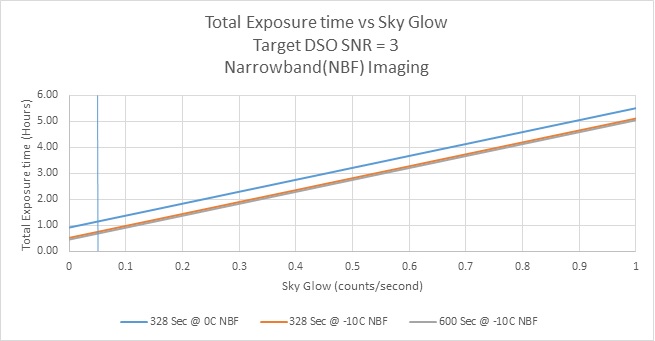
The blue line is for a camera temperature of zero degrees Celsius. The orange line is for a camera temperature of -10 °C. The Pelican Nebula LIGHT frame is a narrowband image, so I believe the DSO rate of 0.05 counts/second best demonstrates the time required to acquire enough data to pull out the faint details in the nebula. An SNR of 3 is low, but the SNR quickly increases for brighter sections of the DSO. The grey line is for a camera temperature of -10 Celsius and an exposure time of 600 seconds, which is the exposure time I would typically use for imaging H-alpha nebulae. In this case, the total exposure time was only slightly reduced. Longer exposures always come with an increased risk of losing an exposure to clouds, bad guiding, etc., so this graph tells me that, for this case, longer exposures are risky with minor improvement in SNR.

I used a thin blue vertical line to indicate the 0.05 count/second Sky Glow that I determined for the Pelican Nebula LIGHT frame. The graph tells me that I could achieve an SNR of 3 after 1.14 hours using a camera temperature of 0 °C. Lowering the camera temperature to -10 °C reduced this time to 0.75 hours. Once the Sky Glow got above 0.7 counts/second, I would need to allocate 4 hours to achieve an SNR of 3. I would conclude that if it’s going to take almost 4 times the total exposure time that the Sky Glow was too much to bother imaging this DSO target.

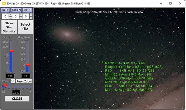
The other filter I use is a BAADER Moon and Skyglow filter. This filter is considered a Light Pollution Filter(LPF). I used this filter for this LIGHT frame from Sept 29th, 2021. It is an image of M110 and a small section of the Andromeda Galaxy(M31). The camera settings were GAIN = 1600, Temperature = -10 Celsius, and Exposure = 300 seconds. I applied a 300-second masterDARK, which eliminated camera BIAS and DARK Current, but leaves Read noise and DARK Current noise in the image. The green rectangle is for a small section of the sky background between these two galaxies. I am going to say that the SD for this small rectangle is 32 counts. The DARK frame Noise Study graph shown at the beginning of this post tells me that the camera noise is 9.6 counts (300 Sec @ -10 Celsius). This means that the noise attributable to the Sky Glow is as follows:

Sky Glow Noise = sqrt(32^2 – 9.6^2) = 30.5 counts ; now convert the Sky Glow Noise to Sky Glow Magnitude
Sky Glow Magnitude = (30.5 x 0.218)^2 / 0.218 = 202.8 counts ; now convert to Sky Glow rate
Sky Glow rate = 202.8 / 300 = 0.68 counts/second

The Sky Glow rate was 0.05 counts/second for the Pelican Nebula image. This is a lot brighter sky, which I primarily attribute to switching from an OPTOLONG LeNhance narrow band filter to the BAADER Moon and Skyglow filter. The BAADER filter lets in a lot more light. This LIGHT frame was taken just outside a big city, so the light pollution was larger. I re-positioned the green rectangle onto a dim section of the Andromeda Galaxy so that I could repeat my DSO analysis for this new target.

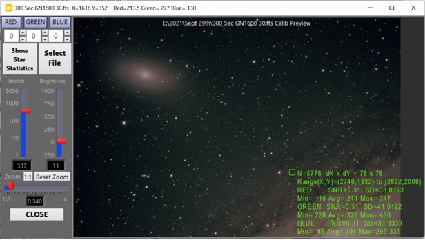
The SD values are now 33.8, 41.0, and 33.3, so I am going to use a value of 35 counts to estimate the total noise. Calculating the DSO noise yields:

DSO noise = sqrt(35^2 – 9.6^2 – 30.5^2) = 14.2 counts ; Now convert DSO noise into DSO magnitude
DSO magnitude = (14.2 *0.218)^2 / 0.218 = 44 counts ; Now convert DSO magnitude into DSO rate
DSO rate = 44 / 300 = 0.147 counts/second

For the Pelican Nebula image, I identified a DSO rate of 0.05 counts/second, so this DSO rate is much higher.

I decided to add a red line to the graph so that I can show how the total exposure time changes when using a light pollution filter(LPF). What makes the difference here is that both the Sky Glow and DSO rates are much higher. I indicated with a vertical red line the 0.68 counts/second Sky Glow rate for the LPF image. The graph indicates it will take only 0.47 hours total exposure time to achieve a stacked SNR of 3 for the dim area of the Andromeda Galaxy indicated by the green box. I was very lucky that night because I was able to get 4.5 hours of total exposure time. I used my SNR equation one last time to determine what the stacked SNR would be for 4.5 hours of total exposure time. It calculated an SNR of 9.24.

What are those SNR values shown on the LIGHT frame statistics?
You may have noticed that buried in the image statistics shown on the various LIGHT frames are SNR values for each pixel color. Here is an example…

N=6720 dX x dY = 84 x 80
Range(X,Y)=(2742,1938) to (2826,2018)
RED SNR=0.28 SD=34.0139
Min= 110 Avg=243.376 Max= 347
GREEN SNR=0.43 SD=40.2456
Min= 239 Avg= 324 Max= 424
BLUE SNR=0.29 SD=33.3333
Min= 82 Avg=194.6 Max=299.333

As you now know, there is a lot of calculation involved in determining SNR and a lot of analysis required to establish Read noise, DARK Current noise, etc. The SNR values shown in the image statistics are an attempt to give an opinion of SNR based upon an approach that doesn’t rely on all this analysis. While the SNR values shown here are related to the actual SNR values, the algorithm used in CaLIGHTs can calculate an SNR value for any image. This gives you the ability to assess whether the SNR is improving as you choose different calibration options. It also allows you to call up the stacked result from Deep Sky Stacker and compare the stacked SNR with the SNR of a single LIGHT frame.

You could say that the SNR values displayed are useful for comparison purposes, but are not absolutely accurate. The SD, Min, Avg, and Max values shown are accurate, and that’s why I used the SD values for this analysis.

Peter